
Date: November 14, 2021
My Teammates
These are the wonderful people that were apart of this awesome project.
Alexia Garces |
Brooke Holyoak |

|

|
Jason Tellez |
Malachi Hale |

|

|
Table of Contents
- Project Planning
- Executive Summary
- Acquire Data
- Prepare Data
- Data Exploration
- Modeling & Evaluation
- Baseline
- Decision Tree
- Random Forest
- K Nearest Neighbors
- Other Models
- Feature Importance
- Modeling with just the top features
- Model Comparison
- Out of Sample Testing
- Modeling the Gender Subsets
- Modeling the Political Party Subsets
- Modeling the Income Level Subsets
- Modeling the Education Level Subsets
- Modeling Takeaways
- Project Delivery
Project Planning
✓ 🟢 Plan ➜ ☐ Acquire ➜ ☐ Prepare ➜ ☐ Explore ➜ ☐ Model ➜ ☐ Deliver
Project Objectives
- Utilize American Trends Panel Datasets (downloadable here), with statistical modeling techniques to assess and attempt to predict sentiment toward particular topics.
- This will culminate into a well-built well-documented jupyter notebook that contains our process and derivation of these predictions.
- Modules will be created that abstract minutiae aspects of the data pipeline process.
Business Goals
- Utilize tabulated statistical data aquired from Pew Research American Trends Surveys.
- Prepare, explore and formulate hypthoesis about the data.
- Build models that can predict future American sentiment toward certain topics, and utilize hyperparameter optimization and feature engineering to improve validation model performance prior to evaluating on test data.
- Document all these steps throughly.
Audience
- General population and individuals without specific knowledge or understanding of the topic or subject.
Deliverables
- A clearly named final notebook. This notebook will contain more detailed processes other than noted within the README and have abstracted scripts to assist on readability.
- A README that explains what the project is, how to reproduce the project, and notes about the project.
- A Python module and associated modules that automate the data acquisition and preparation process.
Executive Summary
- Our team acquired Pew Research Panel survey data and utilized this data to explore the drivers of pessimism in American Prospective Attitudes.
- Being able to understand what most likely drives pessimistic or optimistic thinking about the future will help business leaders clarify strategies for moving foward.
- This project will also help guide expectations of future sucess in the customers these business leaders serve, in addition to the products offered, investment, marketing and sales, and other aspects throughout their organization.
Goals
- Build a model that can predict future American sentiment toward certain topics, utilizing split survey data as the training dataset.
Findings
- Standard demographic features like age, sex, and income are not drivers of overall pessimism. However, features like what will happen to the average family’s standard of living, cost of healthcare, and the future of the public education system are highly correlated to overall pessimism.
Acquire Data
✓ Plan ➜ 🟢 Acquire ➜ ☐ Prepare ➜ ☐ Explore ➜ ☐ Model ➜ ☐ Deliver
- The data is acquired from Pew Research Panel survey data that asks various demographic questions in conjunction with the survey questions themselves.
- The questions all ask for categorical responses from the individuals and the questions pertain to various topics of American life, such as politics and economics.
Working with American Trends Panel Data
Demographic Profile Variables
- Each ATP dataset comes with a number of variables prefixed by “F_” (for “frame”) that contain demographic profile data. These variables are not measured every wave; instead, they are sourced from panel profile surveys conducted on a less frequent basis. Some profile variables are also occasionally asked on panel waves and are accordingly updated for each panelist. Profile information is based on panelists’ most recent response to the profile questions. Some variables are coarsened to help protect the confidentiality of our panelists. Interviewer instructions in
[ ]and voluntary responses in( )are included if the source of a profile variable was ever presented in phone (CATI) mode. See Appendix I for the profile variable codebook.
Unique Identifier
- The variable
QKEYis a unique identifier assigned to each respondent.QKEYcan be used to link multiple panel waves together. Note that except in a few instances,WEIGHT_W41are only provided for single waves. Use caution when analyzing data from multiple waves without weights that are designed for use with multiple waves.
Data Variable Types
- American Trends Panel datasets contain single-punch or multi-punch variables. For questions in a ‘Check all that apply’ format, each option has its own variable indicating whether a respondent selected the item or not. For some datasets there is an additional variable indicating whether a respondent did not select any of the options. Open-end string variables are not included in ATP datasets. Coded responses to open-end questions are included when available.
Dataset Format
- The dataset is formatted as a .sav file and can be read with the SPSS software program. The dataset can also be read with the R programming language, using the
foreignpackage. R is a free, open-source program for statistical analysis that can be downloaded here. It can also be used to export data in .csv format for use with other software programs.
- NOTE: Using other tools to directly convert the .sav file to another format such as .csv may ERASE value labels. For this reason, it is highly recommended that you use either SPSS or R to read the file directly.
DataFrame Dictionary
- Data Dictionary can be viewed here
Takeaways from Acquire:
- We acquired a DataFrame from a Pew Research Panel survey which contained 2524 observations and 124 columns.
- Each row represents an individual American adult and his or her responses to the survey questions.
- Of our 124 columns, 2 are continuous and numeric:
qkeyandweight. The remaining 122 columns are categorical features.
- The
weightcolumn indicates the corresponding survey weight of each respondent in the sample. The survey weight indicates how representative an observation is of the total population.- The survey results provide us with information regarding each respondents’ views about the future of the United States. In addition,the acquired data contains demographic data for each respondent, including gender, race, income level, and political affiliation.
Prepare Data
✓ Plan ➜ ✓ Acquire ➜ 🟢 Prepare ➜ ☐ Explore ➜ ☐ Model ➜ ☐ Deliver
- We will import our
prepare.pyfile, which performs a series of steps to clean and prepare our data:
- First, we convert the categorical features in the DataFrame to objects.
- Second, because our target variable will be the respondents’ prospective thinking, we drop rows for which the respondent refused to answer the question about prospective thinking in the column
OPTIMISMT_W41.
- Third, we rename the columns as indiciated by our data dictionary above.
- Fourth, from the column
OPTIMIST_W41, we create new columnsis_pes,pes_val,is_very_pes, andis_very_opt.
- The column
is_pesintroduces a Boolean value where 1 indicates a pessimistic outlook and is 0 indicates an optimistic outlook.- The column
pes_valranks a respondent’s pessisism, with 0 being the least pessismistic and 3 being the most pessimistic.- The column
is_very_pesintroduces a Boolean value where 1 indicates a very pessimistic outlook and 0 indicates a somewhat pessimistic, somewhat optimistic, or very optimistic outlook.- The column
is_very_optintroduces a Boolean value where 1 indicates a very optimistic outlook and 0 indicates a somewhat optimistic, somewhat pessimistic, or very pessimistic outlook.
- Fifth, we create a
replace_keywhich transforms every response in the categorical columns to a corresponding numeric value. We also introduce arevert_keywhich reverts the numeric values back to the original string responses.
- Finally, we convert the column indicating the unique identity of each respondent
QKEYto an integer.
- Additionally, we split the data into
train,validate, andtestdatasets, stratifying on the target featureis_pes.
Prepare Takeaways
- Utilizing the functions in our
prepare.pywe implemented a series of functions to clean our data.
- We eliminated nine respondents from our dataset because these respondents refused to answer the question
OPTIMIST_W41about prospective thinking of the US’ future.
- Our newly created target feature
is_pesmaps the responses to questionOPTIMIST_W41“Somewhat pessimistic” and “Very pessimistic” as the single Boolean value 1 and the responses “Somewhat optimistic” and “Very optimistic” to the single Boolean value 0.
- Stratifying on
is_pes, we split our data intotrain,validate, andtest, datasets of lengths 1408, 604, and 503, respectively.
Explore Data
✓ Plan ➜ ✓ Acquire ➜ ✓ Prepare ➜ 🟢 Explore ➜ ☐ Model ➜ ☐ Deliver
- We dropped columns that were too closely related to the derivative of our target column (
is_pes):- Those columns ended up being
avg_family,attitude,pes_val,is_very_pesandis_very_opt.- We also dropped
qkeysince it is only an id value and will not provide any information since each is a unique value.- We split our train, validate, and test columns to feature dataframes and target series.
Statistical Test Results
| column_name | chi2 | p_val | deg_free | expected_freq |
|---|---|---|---|---|
happen_general |
309.847 | 5.21955e-68 | 2 | [[ 65.23082386 51.76917614] |
| [299.39275568 237.60724432] | ||||
| [420.37642045 333.62357955]] | ||||
happen_pub_ed |
236.57 | 4.26122e-52 | 2 | [[ 75.26633523 59.73366477] |
| [411.45596591 326.54403409] | ||||
| [298.27769886 236.72230114]] | ||||
happen_child_f2 |
180.023 | 8.72154e-39 | 3 | [[152.76278409 121.23721591] |
| [210.18821023 166.81178977] | ||||
| [ 34.56676136 27.43323864] | ||||
| [387.48224432 307.51775568]] | ||||
happen_race |
157.809 | 5.39807e-35 | 2 | [[317.79119318 252.20880682] |
| [398.07528409 315.92471591] | ||||
| [ 69.13352273 54.86647727]] | ||||
happen_health |
145.05 | 3.18329e-32 | 2 | [[447.6953125 355.3046875 ] |
| [265.94105114 211.05894886] | ||||
| [ 71.36363636 56.63636364]] |
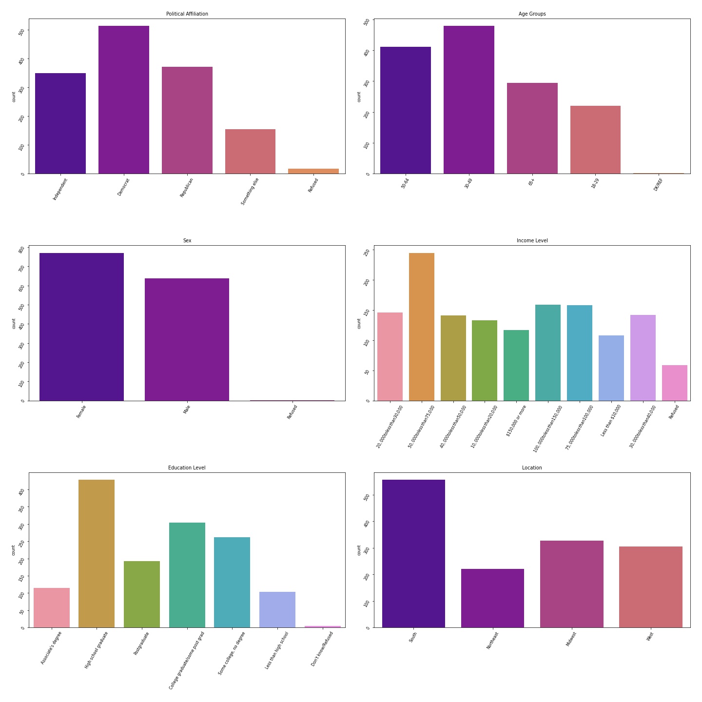
Univariate Distributions
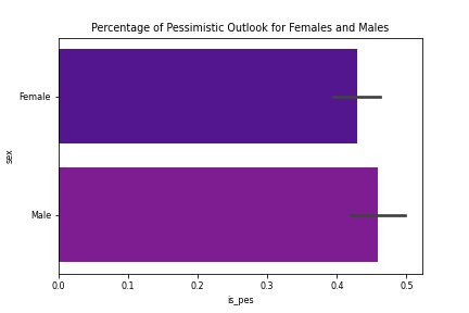
Males vs Females Pessimisim
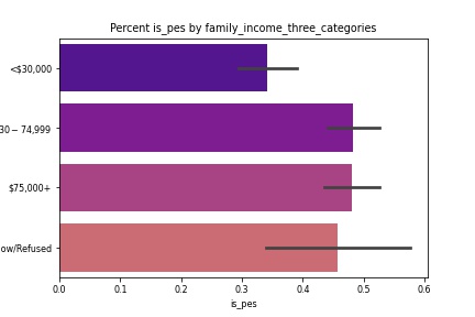
Family Income Pessimisim
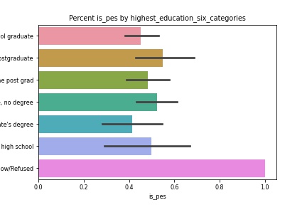
Educational Attainment Pessimisim
Hypotheses & Testing
Hypothesis 1
- H0: Is sex independent of a pessimsitic future outlook?
- Ha: Sex is dependent on pessimist future outlook.
- ɑ: 0.05
Hypothesis 1 Takeaways
- The number of females and males who are overall pessimistic are about the same.
- The p-value is above 0.05, so we accept the null hypothesis.
Hypothesis 2
- H0: Is income independent of a pessimistic future outlook?
- Ha: Income is dependent on pessimistic future outlook.
- ɑ = 0.05
Hypothesis 2 Takeaways
- While it appears that people who are middle income earners are more pessimistic, there is no significance for overall income related to overall pessimism.
- The p-value is above 0.5, so we accept the null hypothesis.
Explore Takeaways
- There a small differences in future outlook when considering sex, income and education.
- While the small differences exist, they do not appear to be significant.
- Through chi-squared testing, we verify that there is not a significant relationship between theses features and our target.
- Even though they are not necessarily drivers of overall future outlook, the findings are still helpful in isolation.
Modeling & Evaluation
✓ Plan ➜ ✓ Acquire ➜ ✓ Prepare ➜ ✓ Explore ➜ 🟢 Model ➜ ☐ Deliver
- We first have to choose a baseline to compare our models against.
- The main models we will be using are Decision Tree, Random Forest, and K-Nearest Neighbor.
- We will use different variations of our models until we determine one model to have outperformed our baseline and to have avoided overfitting or underfitting on the training data.
- We will also be testing feature importance to see what drives an individual’s overall attitude.
- Once we choose our best model, we will run this model on our Out-of-sample dataset.
Baseline
- With a non-pessimistic attitude as our baseline, we calculated our accuracy by asuming that every respondent was non-pressimistic. This method gave us an accuracy of 55.75%.
Decision Tree
- Utilizing the
decision_tree_modelsfunction from ourmodel.pyfile, we created a series of Decision Tree models with varying depths. Using ourtest_a_modelfunction from themodel.py, we calculated the accuracies of these models on thetrainandvalidatedatasets for each of these models.
Random Forest
- Utilizing the
random_forest_modelsfunction from ourmodel.pyfile, we created a series of Random Forest models with varying depths and min samples leaf. Using ourtest_a_modelfunction from themodel.py, we calculated the accuracies of these models on thetrainandvalidatedatasets for each of these models.
K Nearest Neighbors
- Utilizing the
random_forest_modelsfunction from ourmodel.pyfile, we created a series of K Nearest Neighbors models with varying numbers of neighbors. Using ourtest_a_modelfunction from themodel.py, we calculated the accuracies of these models on thetrainandvalidatedatasets for each of these models.
Other Models
- We used the models Linear SVC, Logistic Regression, and Naive Bayes to classifiy pessismistic respondents. We then used the
test_a_modelfunction to evaluate the accuracy of these models on thetrainandvalidatedatasets.
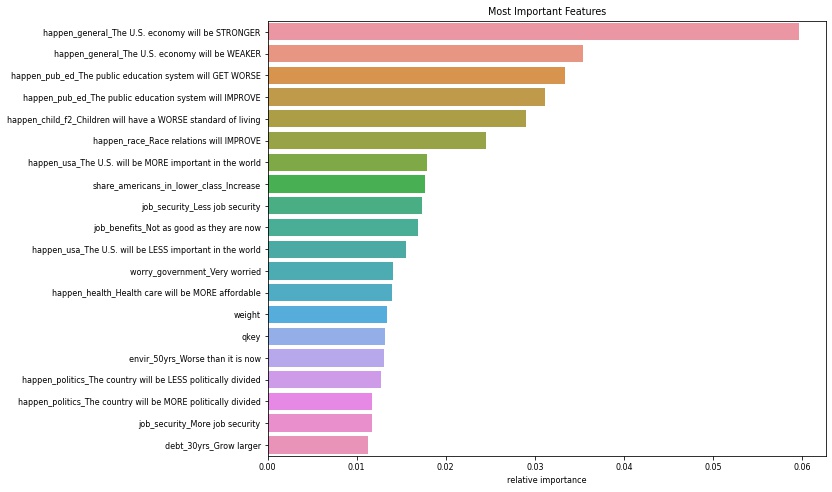
Feature Importance
- Of the models mentioned above, our best performing model was the Random Forest Classifier with depth 8, min samples leaf 3. We utilized this model to perform feature importance on the features in our dataset. We found that public education and U.S. economics are major drivers of pessimism.
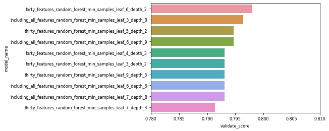
Modeling with just the top features
- Feature importances gave us a ranked order of the features by importance in predicting pessimism. Using these ordered features, we ran a series of Random Forest Classifier models using just the top thirty most important features and just the forty most important features, using varying parameters. None of these models, however, outperformed the the Random Forest Classifier with depth 8, min samples leaf 3 using all features.
Model Comparison
- Our best performing model was the Random Forest Classifier which included all features and had min samples leaf 3 and a depth of 8. This model had an accuracy of 80.46% on the validate dataset.
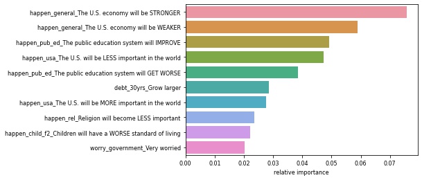
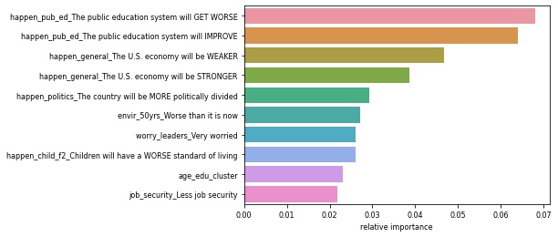
Modeling the Gender Subset
- We ran Random Forest Classification models on the subsets of female and male respondents.
| Most Important Issues For Women | Most Important Issues for Men |
|---|---|
 |
 |
Modeling the Political Party Subsets
- We ran Random Forest Classification models on the subsets of Republican and Democrat respondents.
| Most Important Issues For Republicans | Most Important Issues for Democrats |
|---|---|
 |
 |
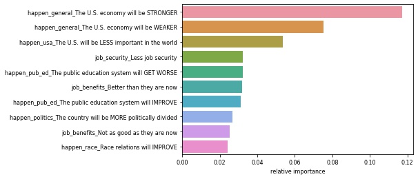
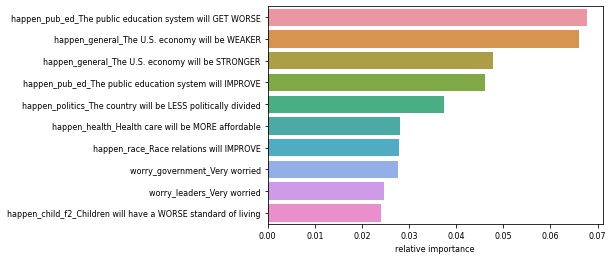
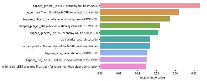
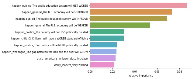
Modeling the Income Level Subsets
- We ran Random Forest Classification models on on the subsets for income groups less than $30,000, between $30,000 and $75,000, and more than $75,000.
| Most Important Issues For Lower Income Level | Most Important Issues for Middle Income Level | Most Important Issues for Upper Income Level |
|---|---|---|
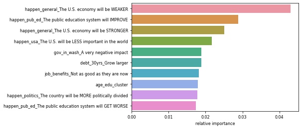 |
 |
 |
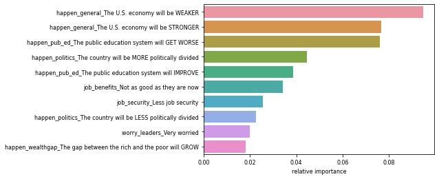
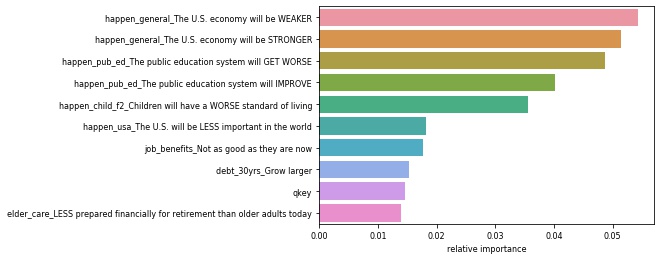
Modeling the Education Level Subsets
- We ran Random Forest Classification models on the subsets for the respondents’ highest education level, grouped by: high school or less, some college, or college graduate and above.
| Most Important Issues For Highest Education High School or Less | Most Important Issues For Highest Education Some College | Most Important Issues For Highest Education College Degree |
|---|---|---|
 |
|
 |
Out of Sample
- We ran our best performing model, selected above on the out-of-sample test dataset. We achieved a 76.54% accuracy.
Modeling Takeaways
- Big drivers of pessimism are public education and economics
- Some other main drivers are job benefits and job security, race relations, standards of living, healthcare, and the country’s world status are also very important to adults
- We chose the most common result of the target column as our baseline with an accuracy of 55.75%.
- We ran over 200 variations of Decision Tree, Random Forest, K-Nearest Neighbor, and other models
- Overall, the model with the best performances was the Random Forest with
max_depth= 8min_samples_leaf= 3- Accuracy:
train(In-sample) = 92.05%validate(Out-of-sample) = 80.46%test(Out-of-sample) = 76.54%
Project Delivery
✓ Plan ➜ ✓ Acquire ➜ ✓ Prepare ➜ ✓ Explore ➜ ✓ Model ➜ 🟢 Deliver
- Currently we are achieving an Out-of-sample accuracy of ~76% on our
testdata and we believe with further feature engineering and hyper-parameter optimization we could achieve a higher accuracy.
Conclusion and Next Steps
- While it appeared that there may have been a significant difference between the genders and their pessimisim, it was not result in this instance.
- Additionally, our other potential observation, that there would be a significant difference in the pessimisim reletive to income, it was again not the result in this instance.
- The next step is to continue finalizing the work and ensuring our work is throughly documented.
- With more time we will continue examining multiple different feature combinations and test for significance from these observations.
Project Replication
- Statistical data can be downloaded from here.
- You can read the SPSS Statistic data file with
pandas.read_spss("ATP W41.sav")
Data Use Agreements
- The source of the data with express reference to the center in accordance with the following citation: “Pew Research Center’s American Trends Panel”
- Any hypothesis, insight and or result within this project in no way implies or suggests as attributing a particular policy or lobbying objective or opinion to the Center, and
- “The opinions expressed herein, including any implications for policy, are those of the author and not of Pew Research Center.”
- Information on The American Trends Panel (ATP) can be found at The American Trends Panel
- More information on these user agreements can be found at Pew Research.
Citation
- “American Trends Panel Wave 41.” Pew Research Center, Washington, D.C. (December 27, 2018).