
Date: October 13, 2021
Table of Contents
Project Planning
✓ 🟢 Plan ➜ ☐ Acquire ➜ ☐ Prepare ➜ ☐ Explore ➜ ☐ Model ➜ ☐ Deliver
Project Objectives
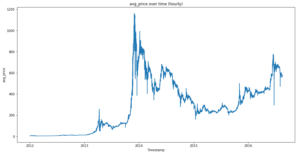
- For this project we will be working with historical price and volume data from Bitcoin between 01-01-2012 & 03-31-2021, these are Bitstamp prices and all are annotated in USD.
- The primary focus is to see if Bitcoin price can be predicted with any reliability or if there is any cyclical observations within Bitcoin pricing or volume.
- The csv data can be downloaded from Kaggle here.
Business Goals
- Create models that are better at predicting Bitcoin price than the baseline.
- Put these models into a Juypter notebook and make the project replicable.
Audience
- Data science professionals as well as any curious cat.
Deliverables
- A clearly named final notebook. This notebook will be what you present and should contain plenty of markdown documentation and cleaned up code.
- A README that explains what the project is, how to reproduce you work, and your notes from project planning.
- A Python module or modules that automate the data acquisistion and preparation process. These modules should be imported and used in your final notebook.
Executive Summary
Goals
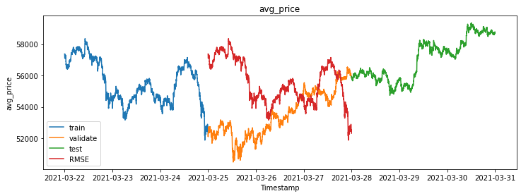
- This project is to utilize machine learning modeling to predict the avgerage price of Bitcoin, better than the baseline.
- Abstract the functions to sub python scripts to have a clean presentation, and throughly document.
Findings
- The dataset had quite a few null values, but utilizing a forward fill method offered an easy and effective remedy. Otherwise, this dataset was quite clean.
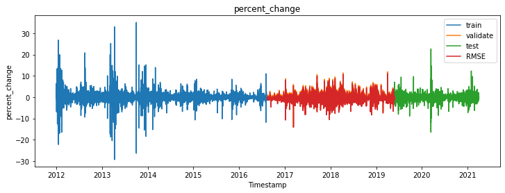
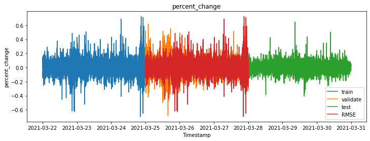
- Another key aspect of predicting Bitcoin’s price was the percent change within a time interval.
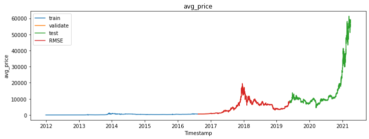
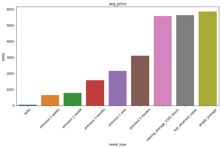
- The best performing model was Holt’s Linear Trend that was fine tuned for the dataset via slope and level smoothness, with an RMSE of 53.
Acquire Data
✓ Plan ➜ 🟢 Acquire ➜ ☐ Prepare ➜ ☐ Explore ➜ ☐ Model ➜ ☐ Deliver
Data Tail
| Timestamp | Open | High | Low | Close | Volume_(BTC) | Volume_(Currency) | Weighted_Price |
|---|---|---|---|---|---|---|---|
| 2021-03-30 23:56:00 | 58714.3 | 58714.3 | 58686 | 58686 | 1.38449 | 81259.4 | 58692.8 |
| 2021-03-30 23:57:00 | 58684 | 58693.4 | 58684 | 58685.8 | 7.29485 | 428158 | 58693.2 |
| 2021-03-30 23:58:00 | 58693.4 | 58723.8 | 58693.4 | 58723.8 | 1.70568 | 100117 | 58696.2 |
| 2021-03-30 23:59:00 | 58742.2 | 58770.4 | 58742.2 | 58760.6 | 0.720415 | 42333 | 58761.9 |
| 2021-03-31 00:00:00 | 58767.8 | 58778.2 | 58756 | 58778.2 | 2.71283 | 159418 | 58764.3 |
Data Dictonary
| Feature | Datatype | Definition |
|---|---|---|
| Timestamp | 4857377 non-null: datetime64[ns] | start tiem of time window (60s window), in Unix Time |
| Open | 3613769 non-null: float64 | Open price at start time window |
| High | 3613769 non-null: float64 | High price within the time window |
| Low | 3613769 non-null: float64 | Low price within the time window |
| Close | 3613769 non-null: float64 | Close price at the end of the time window |
| Volume_(BTC) | 3613769 non-null: float64 | Volume of BTC transacted in this window |
| Volume_(Currency) | 3613769 non-null: float64 | Volume of corresponding currency transacted in this window |
| Weighted_Price | 3613769 non-null: float64 | VWAP - Volume Weighted Average Price |
Takeaways from Acquire:
- Target variable:
avg_price- This dataframe currenly has 4,857,377 rows and 8 columns
- There are 1,243,608 missing values.
- All columns are float64 types of data.
Prepare Data
✓ Plan ➜ ✓ Acquire ➜ 🟢 Prepare ➜ ☐ Explore ➜ ☐ Model ➜ ☐ Deliver
- Add additional columns of
month,day_of_week,price_diff,price_delta,percent_changeandday_num.- Filling the null values with the most recent value will likely be the best course of action.
New Data Dictionary
| Feature | Datatype | Definition |
|---|---|---|
| Open | 4857377 non-null: float64 | Open price at start time window |
| High | 4857377 non-null: float64 | High price within the time window |
| Low | 4857377 non-null: float64 | Low price within the time window |
| Close | 4857377 non-null: float64 | Close price at the end of the time window |
| Volume_(BTC) | 4857377 non-null: float64 | Volume of BTC transacted in this window |
| Volume_(Currency) | 4857377 non-null: float64 | Volume of corresponding currency transacted in this window |
| Weighted_Price | 4857377 non-null: float64 | VWAP - Volume Weighted Average Price |
| day_of_week | 4857377 non-null: object | Verbose name of the week |
| day_of_week_num | 4857377 non-null: int64 | number representing the day of the week |
| month | 4857377 non-null: object | Month number and month name |
| month_num | 4857377 non-null: int64 | number representing the month of the year |
| price_diff | 4857377 non-null: float64 | Delta between the Close and Open (Close - Open) |
| price_delta | 4857377 non-null: float64 | Delta between the High and Low (High - Low) |
| day_num | 4857377 non-null: int64 | The numeric number of the day of the month |
| avg_price | 4857377 non-null: float64 | Avg price for the time period ([Open + Close] / 2) |
| percent_change | 4857377 non-null: float64 | Price difference / Open price represented as a percentage (price_diff / Open) |
Prepare Takeaways
- The data is now prepared to be input into the explore aspects of the data pipeline to evaluate what features we should use to potentially run time-series analysis on.
Explore Data
✓ Plan ➜ ✓ Acquire ➜ ✓ Prepare ➜ 🟢 Explore ➜ ☐ Model ➜ ☐ Deliver
Bitcoin Price over Time
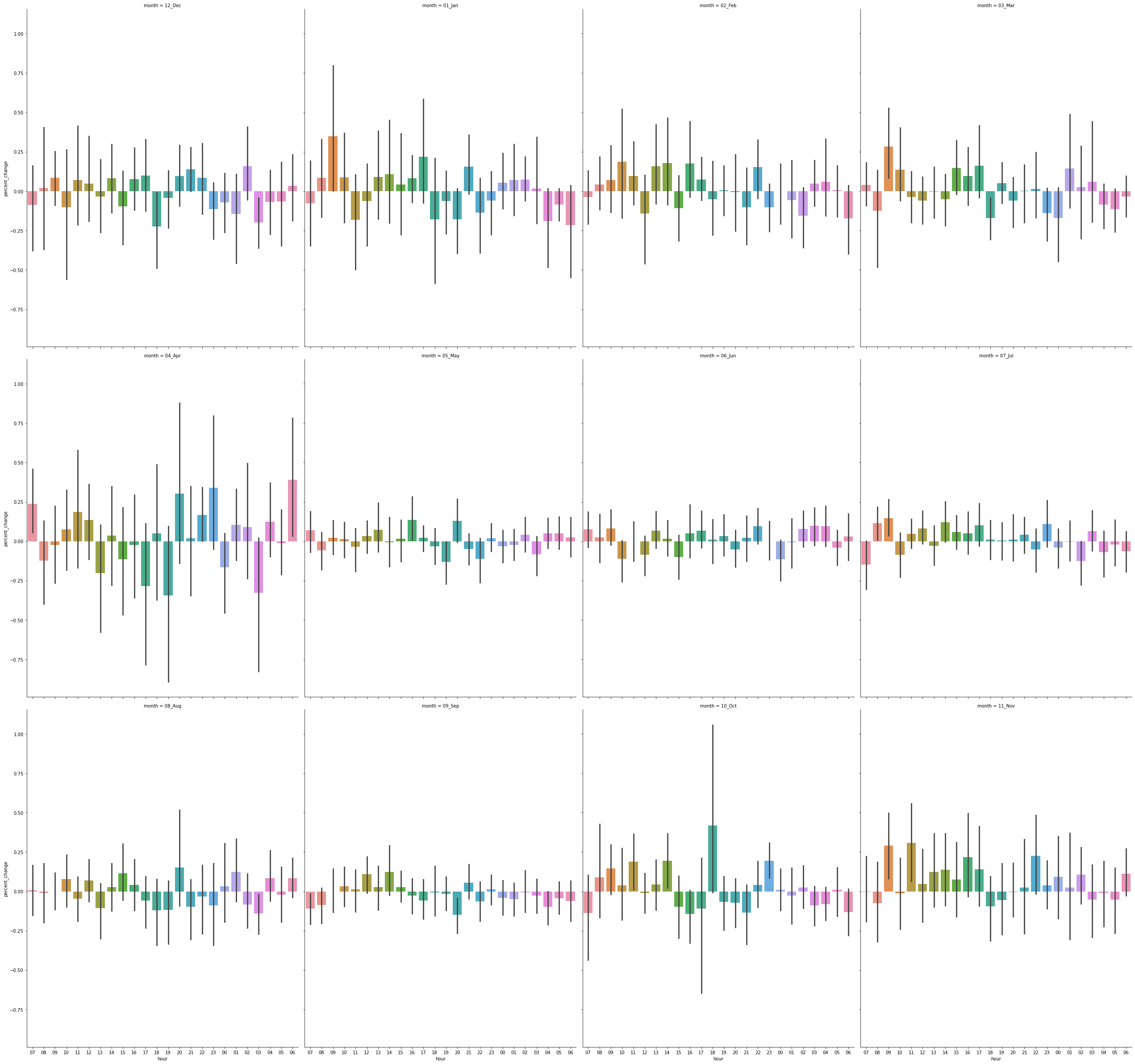
Hour vs Percent Change on a monthly basis
Correlations
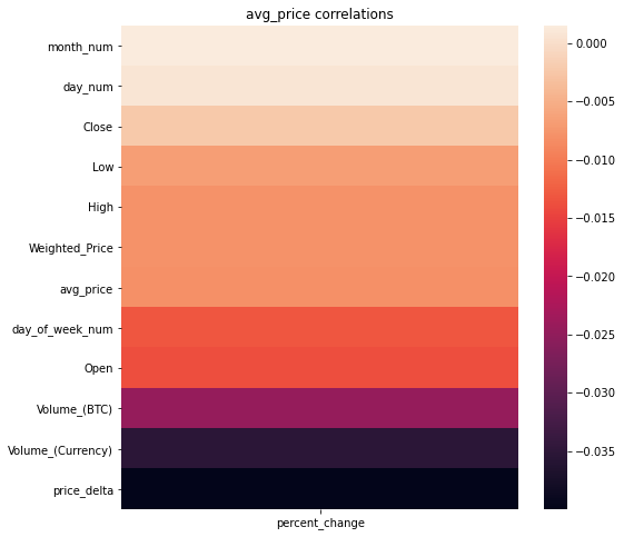
Correlations of Average Price
| Column Name | avg_price |
|---|---|
| price_diff | 0.0061726 |
| percent_change | 0.00543991 |
| Volume_(Currency) | -0.0475418 |
| Volume_(BTC) | -0.067203 |
| price_delta | -0.142155 |
| day_num | -0.346819 |
| month_num | nan |
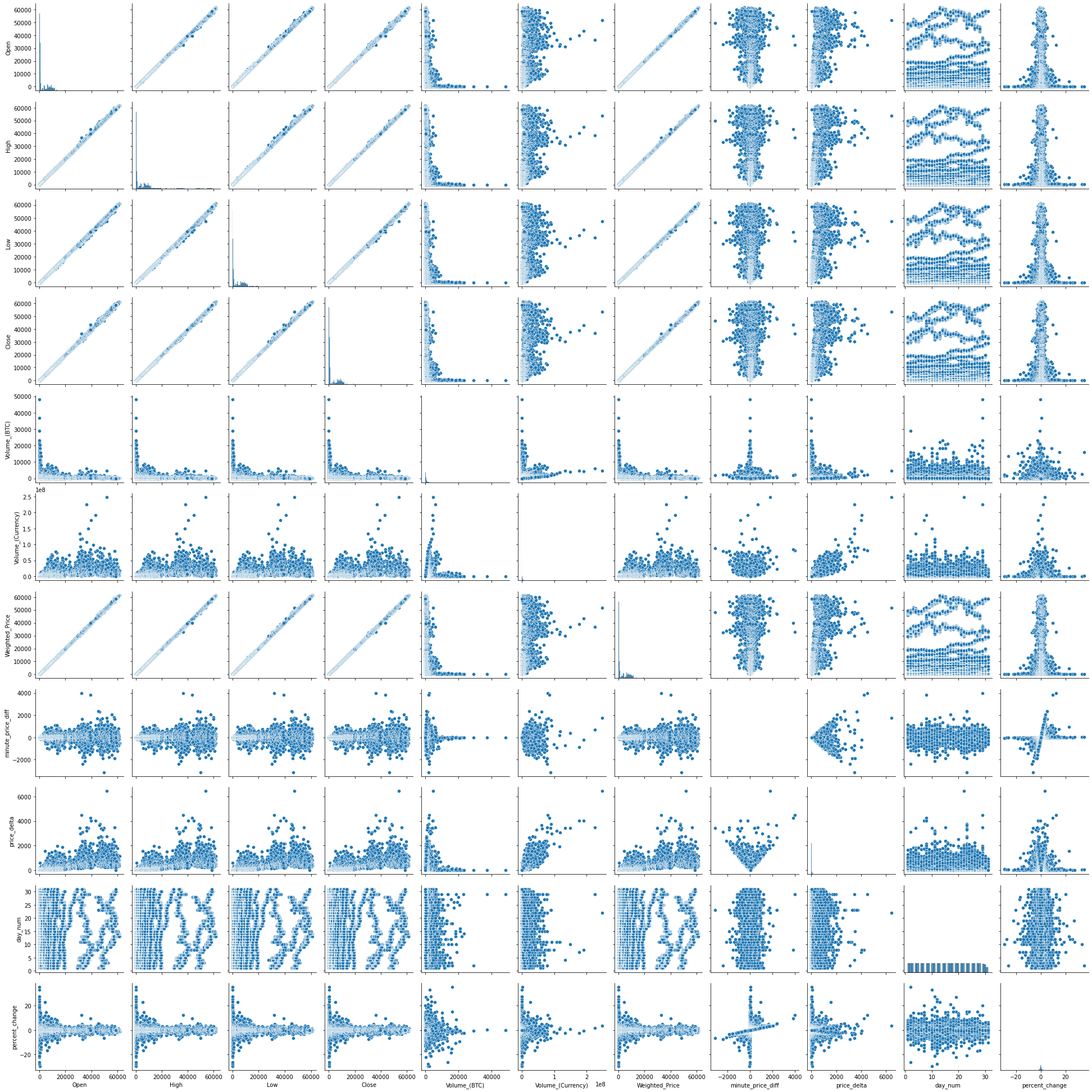
Pair Plot
Explore Takeaways
- It is apparent that the most correlated features with
avg_priceareday_num,price_delta,Volume_(BTC).- It also appears that the avg_price tends to trend upward during Oct, and downwards in Sept.
Modeling
✓ Plan ➜ ✓ Acquire ➜ ✓ Prepare ➜ ✓ Explore ➜ 🟢 Model ➜ ☐ Deliver
Last Observed Value
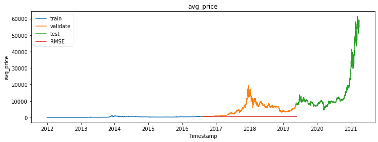
Average Price

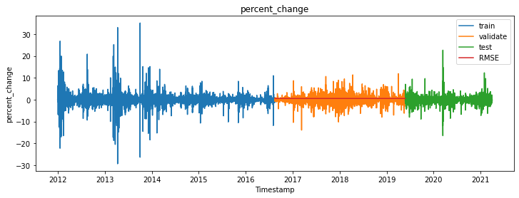
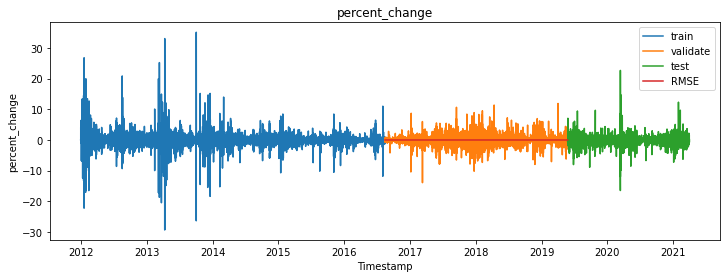
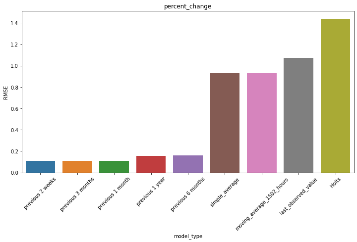
Percent Change
Rolling/Moving Average
Average Price
Percent Change
Holt’s Linear Trend
Average Price
Percent Change
Previous Cycle (6 months)
Average Price
Percent Change
Project Delivery
✓ Plan ➜ ✓ Acquire ➜ ✓ Prepare ➜ ✓ Explore ➜ ✓ Model ➜ 🟢 Deliver
Root Mean Square Deviation Results
Average Price
Percent Change
Conclusions & Next Steps
- I found that there were large variations in certain models RMSE but the models that could be tuned (such as Holt’s and Previous Cycles) performed best after optimization.
- If I had more time to work on this project, I’d continue doing more performance tuning and possibly aggregating other external data factors that could provide a higher level of correlation or model accuracy.
Replication
- Download the the csv data from Kaggle here.
- Download the
acquire.py&prepare.pyfiles and then run the final notebook.